Graph User Manual

Graph ► Tasks ► Set Of 2D Points

The Set Of 2D Points task plots curves, well not really. The longer explanation is that it plots sets of sequences of pairs of scalars, but saying it plots curves is a lot easier. It also makes scatter plots and area graphs. By applying an appropriate skin using the Edit Graph tool it can also plot trajectories. Here are a few notes regarding this task:

Data is defined like this: { {p_1,1, p_2,1, ... p_n1,1} , {p_1,2, p_2,2, ... p_n2,2} ... {p_1,m, p_2,m, ... p_nm,m} }. Translation: Form a sequence of 2D points (denoted by p_i,j where i is the sequence index and p_i,j is a pair of scalars {x_i,j, y_i,j}) and then form a sequence of sequence of points (where j is the set element index and an element of the set is a sequence of points). The "sequence of points" is called simply "2D Points" or an element of the set of points, hence the name Set Of 2D Points. An element is defined as a particular sequence in the set.
Data are not entered in set or sequence notation. Rather each sequence of points are entered separately as a list of delimited pairs of numbers.
Curves are formed from each sequence of points and multiple curves are implemented by elements of the set.
The word "curve" is simply a convenience and does not indicate that a curve is defined. Curve is simply easier to understand.
There is no enforcement of ascending x values in the numeric views, however when a curve is plotted then the points will be reordered to make x ascending. Scatter plots do not impose that restriction since they are not x or y ordered.
Touching a curve or data point shows its values. Touch-drag over the chart scans one group of data (curve) at a time.
For date entry see Date Graph.
The Bubble Graph section explains how to add and display arbitrary labels at each data point and how to add and display another dimension.

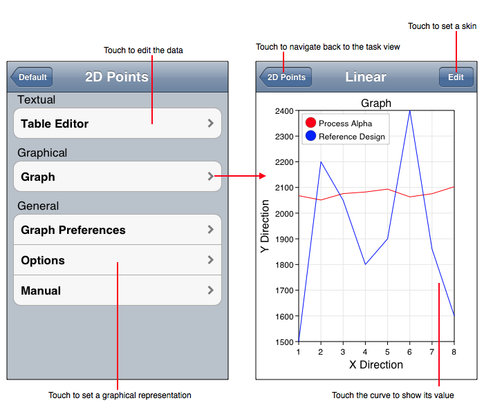
The figure below diagrams the Set Of 2D Points task.

Data Importing and Exporting Formats

The Table Editor atomic cell type is a 2D Point, that is two scalars interpreted as the x-value and then y-value. The component cell type is a scalar representing x-values for odd numbered columns and y-values for even numbered columns. The column, row and block-select import format is a list of 2D Points separated by a delimiter for atomic cells and scalars for component cells.
For the Edit Data (available in Developer Mode only) tool each curve (point sequence) is entered by first assigning a number from 1-20 in the Textual row entry (corresponding to the element index in the set) and then navigating to that curve's editing tool. 1 is the default and will do for a simple line graph. The format is a list of pair of numbers (2D points) separated by a blank.
The Fetch Data format is a list of pair of numbers (2D points) separated by a blank or an XML structure.

Representations

The Set Of 2D Points tasks implements the representations described in the following table. Remember that Skins can affect the representation and may even alter the representation to not conform to the following descriptions.

Representation	Description
Curve > Linear	Shows a usual line graph which is on a rectilinear (Cartesian, x-y) coordinate system. A line graph can have multiple curves on it. X values are reordered as needed to be ascending.
Curve > Semi-Log	Same as Curve > Linear except the coordinate system (and hence the graph) is semi log which means x-linear y-log. The log autoscalar is set to use full cycle or sub cycle log increments as needed to satisfy the data. Use Skins to change the plethora of autoscale parameters or to turn the autoscaler off. IMPORTANT: x and y are input in linear units and are presented on the log scale, do not enter log(y) values and expect things to work out.
Curve > X-Log	Same as Curve > Semi-Log except x-log y-linear coordinates.
Curve > Log-Log	Same as Curve > Semi-Log except x-log y-log coordinates.
Curve > Polar	Same as Curve > Linear except the data is shown on a polar coordinate system where x is interpreted as Θ and y as radius, i.e.: x and y are not transformed (via r = sqrt(x² + y²), Θ = arctan(y/x) ) but rather are interpreted as the independent variables of the coordinate system which means x = &Theta and y = radius. Also note that this graph representation is not a true polar coordinate system as the origin is not zero but rather defined by the autoscalar and minimum r data value. To set the origin to zero use a Skins and turn the r-minimum autoscalar off and the limit value to zero. You can also fix the theta limits so that the coordinate system is shown by a partial polar grid, such as a semi-circular polar grid.
Curve > R-Log	Same as Curve > Polar except the r direction is a log scale not linear. Note that the origin is not zero as is required by log scales. Also note that the autoscalar will use sub or full cycle representations as needed.
Curve > Date	Same as Curve > Linear except the coordinate system (and hence the graph) is x-date y-linear. To enter dates see the Date Graph support section.
Area > Linear	Same as Curve > Linear except the area under the curve is filled in with a color, that is between y and y=0 so for y < 0 the area under the curve is actually above the curve. If y = 0 is not within the graph frame as when the y-axis minimum is greater than 0 then the area extends out of the graph frame. To accommodate that issue the clipping frame is turned on. Use a Skins to turn the clipping off if needed.
Area > Semi-Log	Same as Curve > Semi-Log except the area under the curve to the y-minimum frame value of the graph is filled with the expectation that it signifies the entire area under the curve.
Area > X-Log	Same as Curve > X-Log except the area under the curve to the y-minimum frame value of the graph is filled with the expectation that it signifies the entire area under the curve.
Area > Log-Log	Same as Curve > Log-Log except the area under the curve to the y-minimum frame value of the graph is filled with the expectation that it signifies the entire area under the curve.
Area > Polar	Same as Curve > Polar except the area from the r values of the curve to the origin of the coordinate system is filled in.
Area > R-Log	Same as Curve > R-Log except the area from the r values of the curve to the origin of the coordinate system is filled in.
Scatter > Linear	Same as Curve > Linear except the curve is now designated by circles at each point without interpolating line segments. Use Skins to change the circle to nearly anything and also to turn on the interpolating line segment and thus make a scatter plot into a trajectory plot.
Scatter > Semi-Log	Same as Scatter > Linear except the coordinate system is x-linear, y-log.
Scatter > X-Log	Same as Scatter > Linear except the coordinate system is x-log, y-linear.
Scatter > Log-Log	Same as Scatter > Linear except the coordinate system is x-log, y-log.
Scatter > Polar	Same as Scatter > Linear except the coordinate system is Θ, R. The information for Curve > Polar also applies
Scatter > R-Log	Same as Scatter > Linear except the coordinate system is Θ, R-log. The information for Curve > R-Log also applies.

© Copyright 1993-2021 by VVimaging, Inc. (VVI); All Rights Reserved. Please email support@vvi.com with any comments you have concerning this documentation. See Legal for trademark and legal information.